Topic Modeling in Python using LDA (Latent Dirichlet Allocation)
Introduction
Topic Models, in a nutshell, are a type of statistical language models used for uncovering hidden structure in a collection of texts. In a practical and more intuitively, you can think of it as a task of:
Dimensionality Reduction, where rather than representing a text T in its feature space as {Word_i: count(Word_i, T) for Word_i in Vocabulary}, you can represent it in a topic space as {Topic_i: Weight(Topic_i, T) for Topic_i in Topics}
Unsupervised Learning, where it can be compared to clustering, as in the case of clustering, the number of topics, like the number of clusters, is an output parameter. By doing topic modeling, we build clusters of words rather than clusters of texts. A text is thus a mixture of all the topics, each having a specific weight
Tagging, abstract “topics” that occur in a collection of documents that best represents the information in them.
There are several existing algorithms you can use to perform the topic modeling. The most common of it are, Latent Semantic Analysis (LSA/LSI), Probabilistic Latent Semantic Analysis (pLSA), and Latent Dirichlet Allocation (LDA)
In this article, we’ll take a closer look at LDA, and implement our first topic model using the sklearn implementation in python 2.7
Theoretical Overview
LDA is a generative probabilistic model that assumes each topic is a mixture over an underlying set of words, and each document is a mixture of over a set of topic probabilities.

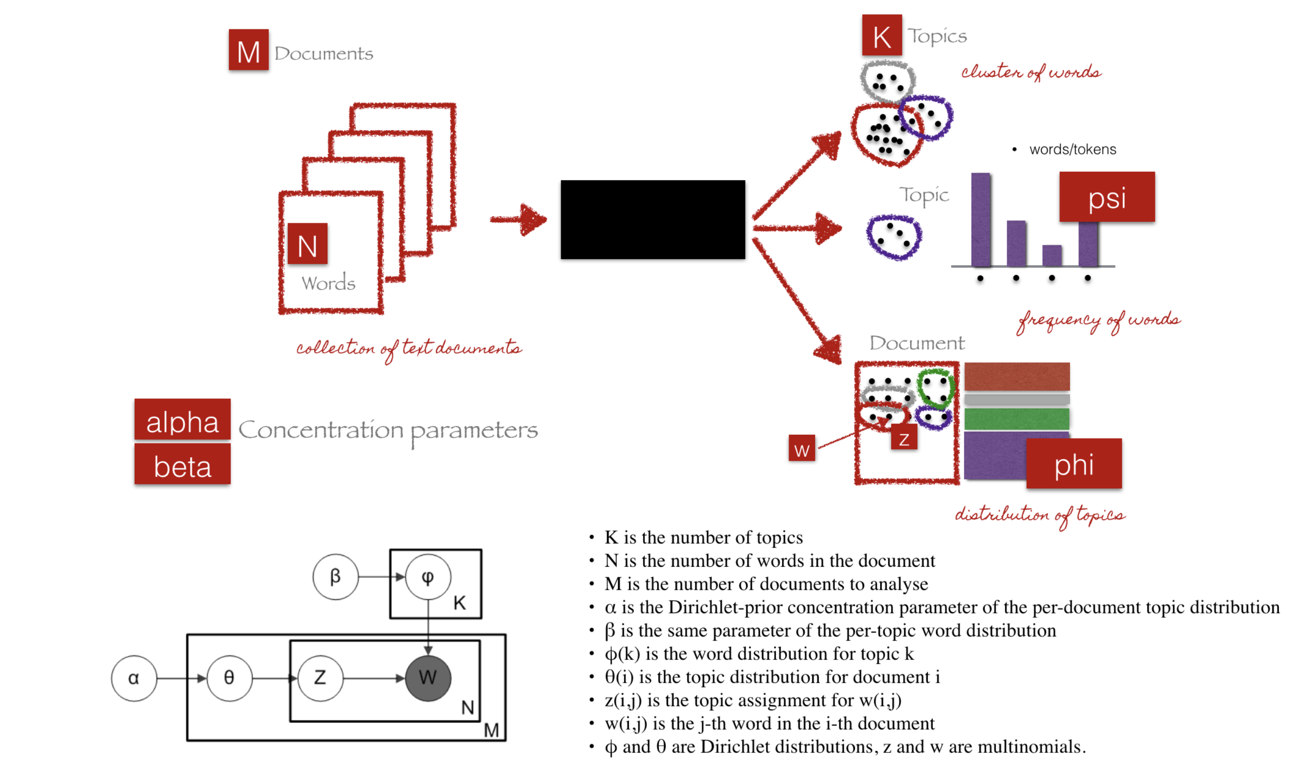
We can describe the generative process of LDA as, given the M number of documents, N number of words, and prior K number of topics, the model trains to output:
psi, the distribution of words for each topic K
phi, the distribution of topics for each document i
Parameters of LDA
Alpha parameter is Dirichlet prior concentration parameter that represents document-topic density — with a higher alpha, documents are assumed to be made up of more topics and result in more specific topic distribution per document.
Beta parameter is the same prior concentration parameter that represents topic-word density — with high beta, topics are assumed to made of up most of the words and result in a more specific word distribution per topic.
LDA Implementation
The complete code is available as a Jupyter Notebook on GitHub
- Loading data
- Data cleaning
- Exploratory analysis
- Preparing data for LDA analysis
- LDA model training
- Analyzing LDA model results
Loading data
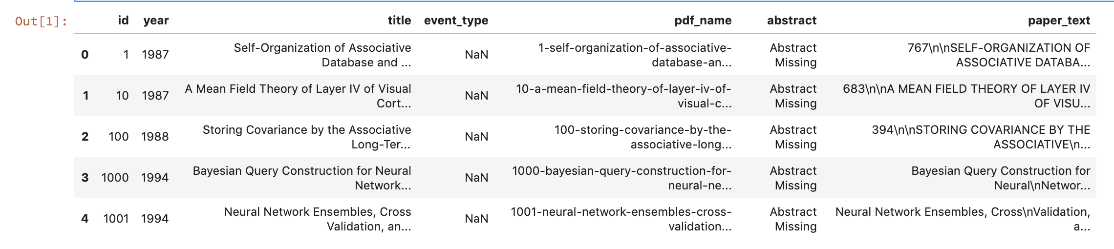
For this tutorial, we’ll use the dataset of papers published in NIPS conference. The NIPS conference (Neural Information Processing Systems) is one of the most prestigious yearly events in the machine learning community. The CSV data file contains information on the different NIPS papers that were published from 1987 until 2016 (29 years!). These papers discuss a wide variety of topics in machine learning, from neural networks to optimization methods, and many more.
Let’s start by looking at the content of the file
# Importing modules
import pandas as pd
import osos.chdir('..')# Read data into papers
papers = pd.read_csv('./data/NIPS Papers/papers.csv')# Print head
papers.head()

Data Cleaning
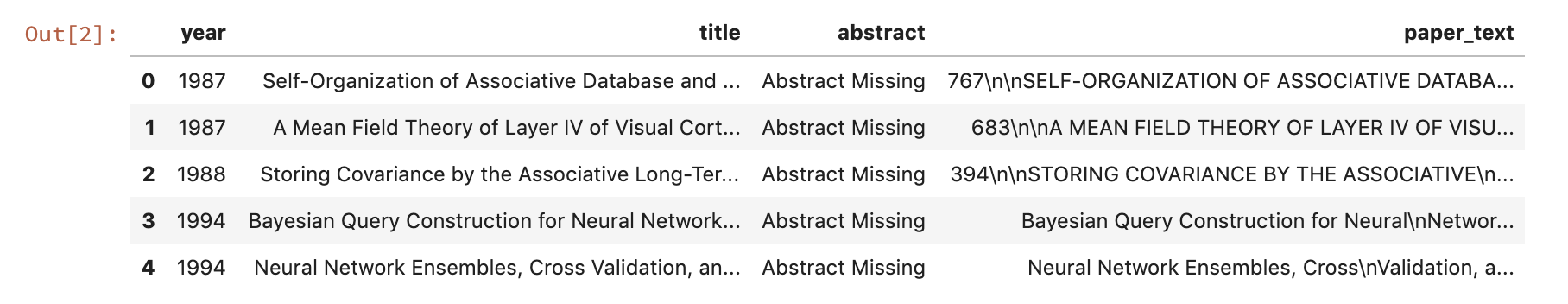
Since the goal of this analysis is to perform topic modeling, we will solely focus on the text data from each paper, and drop other metadata columns
# Remove the columns
papers = papers.drop(columns=['id', 'event_type', 'pdf_name'], axis=1)# Print out the first rows of papers
papers.head()

Remove punctuation/lower casing
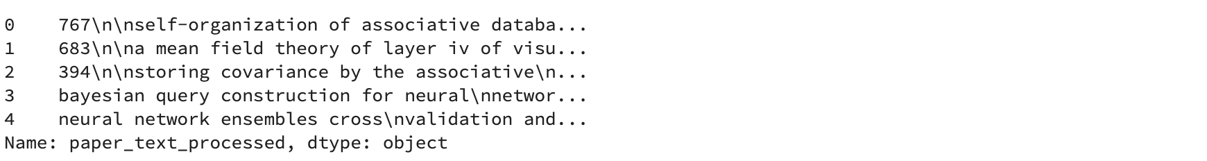
Next, let’s perform a simple preprocessing on the content of paper_text column to make them more amenable for analysis, and reliable results. To do that, we’ll use a regular expression to remove any punctuation, and then lowercase the text
# Load the regular expression library
import re# Remove punctuation
papers['paper_text_processed'] = papers['paper_text'].map(lambda x: re.sub('[,\.!?]', '', x))# Convert the titles to lowercase
papers['paper_text_processed'] = papers['paper_text_processed'].map(lambda x: x.lower())# Print out the first rows of papers
papers['paper_text_processed'].head()

Exploratory Analysis
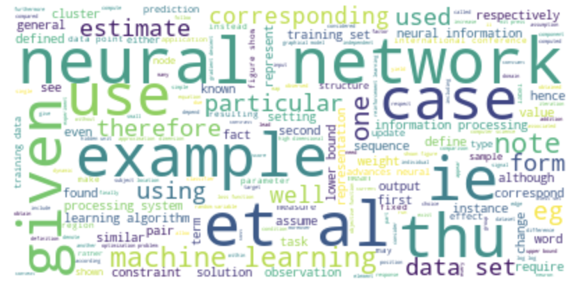
To verify whether the preprocessing happened correctly, we’ll make a word cloud using the wordcloud package to get a visual representation of most common words. It is key to understanding the data and ensuring we are on the right track, and if any more preprocessing is necessary before training the model.
# Import the wordcloud library
from wordcloud import WordCloud# Join the different processed titles together.
long_string = ','.join(list(papers['paper_text_processed'].values))# Create a WordCloud object
wordcloud = WordCloud(background_color="white", max_words=5000, contour_width=3, contour_color='steelblue')# Generate a word cloud
wordcloud.generate(long_string)# Visualize the word cloud
wordcloud.to_image()

Prepare text for LDA Analysis
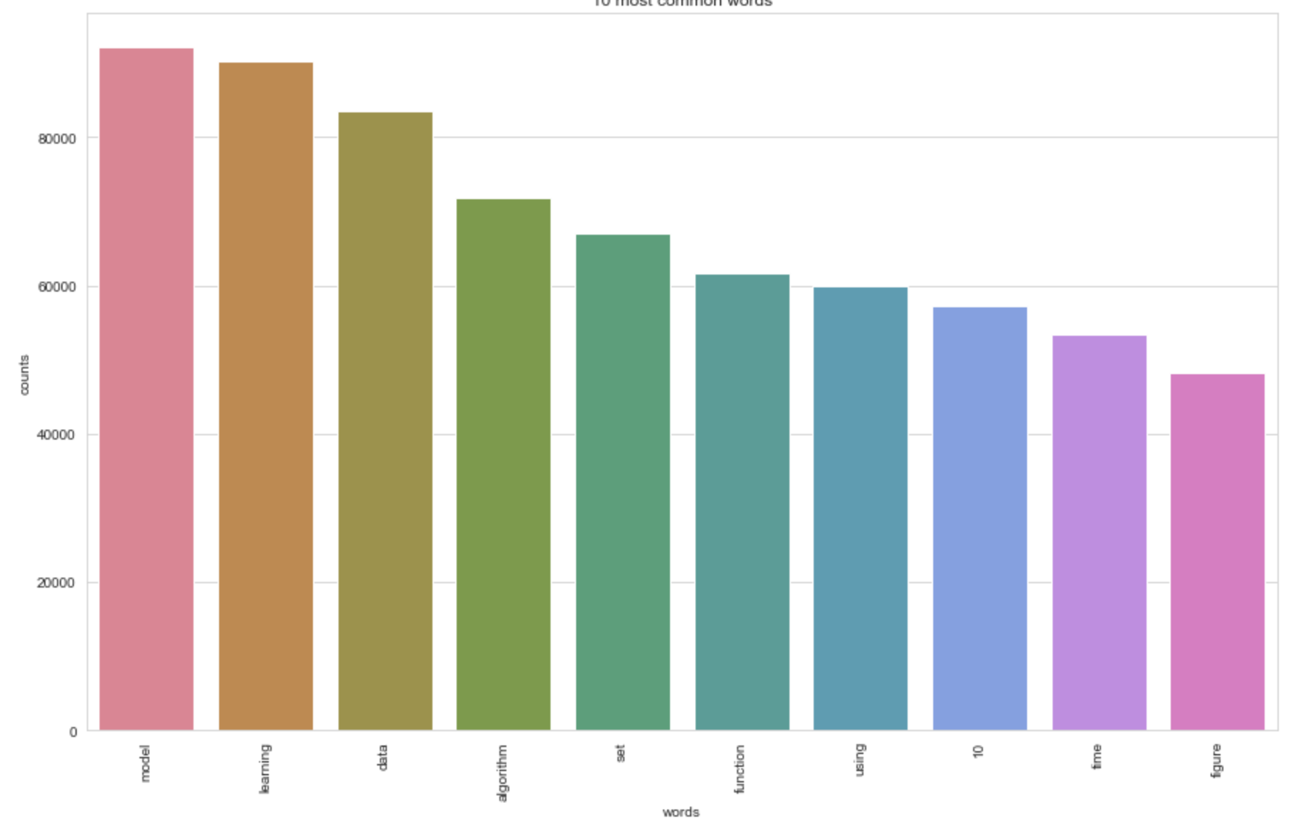
Next, let’s work to transform the textual data in a format that will serve as an input for training LDA model. We start by converting the documents into a simple vector representation (Bag of Words BOW). Next, we will convert a list of titles into lists of vectors, all with length equal to the vocabulary.
We’ll then plot the ten most frequent words based on the outcome of this operation (the list of document vectors). As a check, these words should also occur in the word cloud.
# Load the library with the CountVectorizer method
from sklearn.feature_extraction.text import CountVectorizer
import numpy as npimport matplotlib.pyplot as plt
import seaborn as sns
sns.set_style('whitegrid')
%matplotlib inline# Helper function
def plot_10_most_common_words(count_data, count_vectorizer):
    import matplotlib.pyplot as plt
    words = count_vectorizer.get_feature_names()
    total_counts = np.zeros(len(words))
    for t in count_data:
        total_counts+=t.toarray()[0]

    count_dict = (zip(words, total_counts))
    count_dict = sorted(count_dict, key=lambda x:x[1], reverse=True)[0:10]
    words = [w[0] for w in count_dict]
    counts = [w[1] for w in count_dict]
    x_pos = np.arange(len(words))

    plt.figure(2, figsize=(15, 15/1.6180))
    plt.subplot(title='10 most common words')
    sns.set_context("notebook", font_scale=1.25, rc={"lines.linewidth": 2.5})
    sns.barplot(x_pos, counts, palette='husl')
    plt.xticks(x_pos, words, rotation=90)
    plt.xlabel('words')
    plt.ylabel('counts')
    plt.show()# Initialise the count vectorizer with the English stop words
count_vectorizer = CountVectorizer(stop_words='english')# Fit and transform the processed titles
count_data = count_vectorizer.fit_transform(papers['paper_text_processed'])# Visualise the 10 most common words
plot_10_most_common_words(count_data, count_vectorizer)

LDA model training and results visualization
To keep things simple, we will only tweak the number of topic parameters.
import warnings
warnings.simplefilter("ignore", DeprecationWarning)# Load the LDA model from sk-learn
from sklearn.decomposition import LatentDirichletAllocation as LDA
# Helper function
def print_topics(model, count_vectorizer, n_top_words):
words = count_vectorizer.get_feature_names()
for topic_idx, topic in enumerate(model.components_):
print("\nTopic #%d:" % topic_idx)
print(" ".join([words[i]
for i in topic.argsort()[:-n_top_words - 1:-1]]))
# Tweak the two parameters below
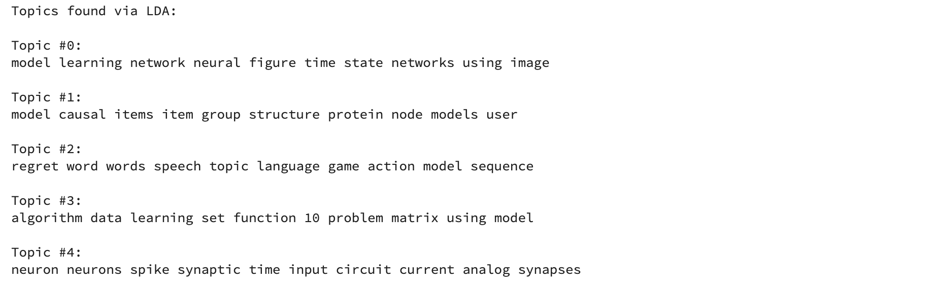
number_topics = 5
number_words = 10# Create and fit the LDA model
lda = LDA(n_components=number_topics, n_jobs=-1)
lda.fit(count_data)# Print the topics found by the LDA model
print("Topics found via LDA:")
print_topics(lda, count_vectorizer, number_words)

Analyzing LDA model results
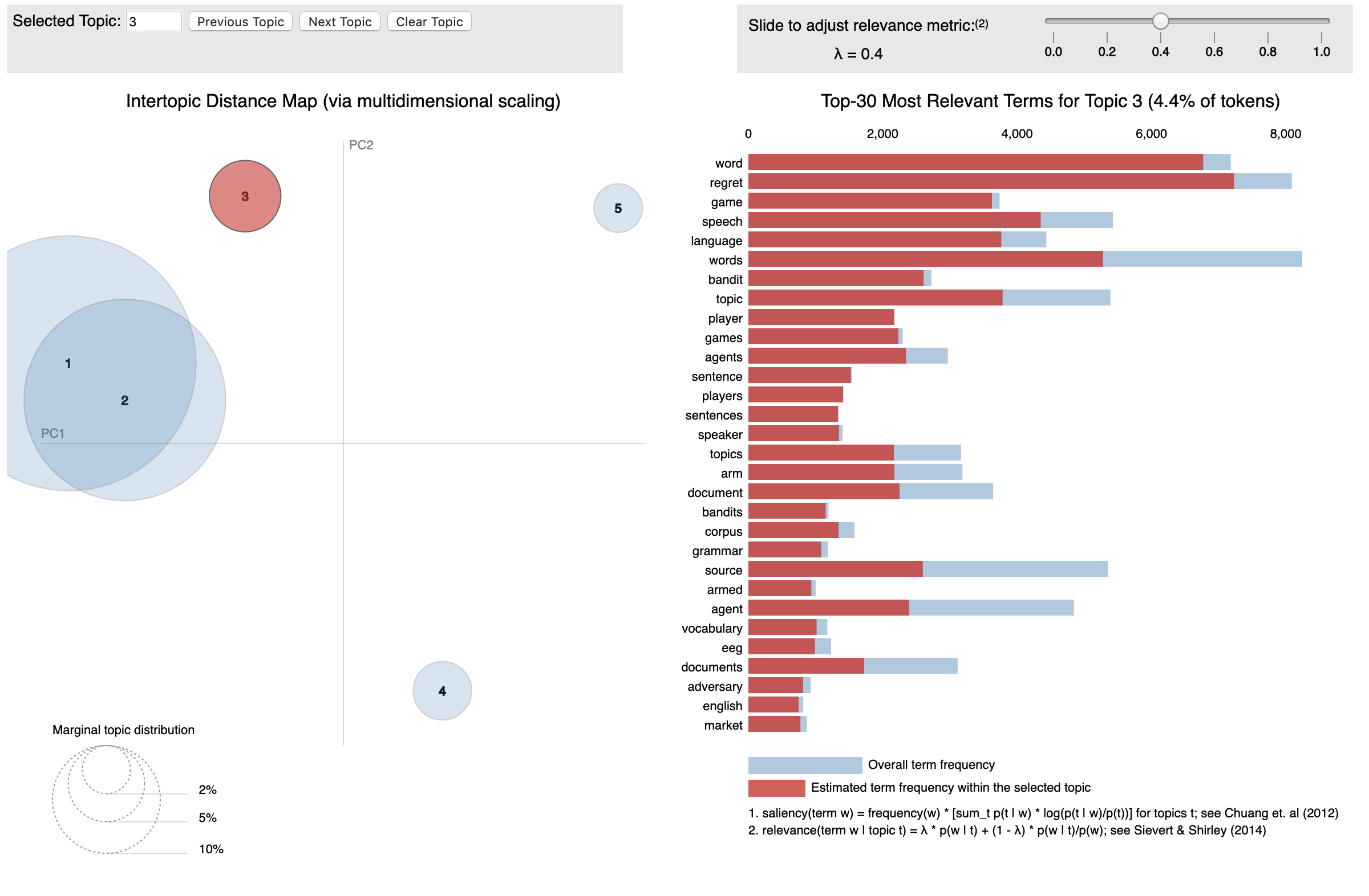
Now that we have a trained model let’s visualize the topics for interpretability. To do so, we’ll use a popular visualization package, pyLDAvis which is designed to help interactively with:
- Better understanding and interpreting individual topics, and
- Better understanding the relationships between the topics.
For (1), you can manually select each topic to view its top most frequent and/or “relevant” terms, using different values of the λ parameter. This can help when you’re trying to assign a human interpretable name or “meaning” to each topic.
For (2), exploring the Intertopic Distance Plot can help you learn about how topics relate to each other, including potential higher-level structure between groups of topics.
%%time
from pyLDAvis import sklearn as sklearn_lda
import pickle
import pyLDAvisLDAvis_data_filepath = os.path.join('./ldavis_prepared_'+str(number_topics))
# # this is a bit time consuming - make the if statement True
# # if you want to execute visualization prep yourself
if 1 == 1:LDAvis_prepared = sklearn_lda.prepare(lda, count_data, count_vectorizer)with open(LDAvis_data_filepath, 'w') as f:
        pickle.dump(LDAvis_prepared, f)

# load the pre-prepared pyLDAvis data from disk
with open(LDAvis_data_filepath) as f:
    LDAvis_prepared = pickle.load(f)pyLDAvis.save_html(LDAvis_prepared, './ldavis_prepared_'+ str(number_topics) +'.html')

Closing Notes
Machine learning has become increasingly popular over the past decade, and recent advances in computational availability have led to exponential growth to people looking for ways how new methods can be incorporated to advance the field of Natural Language Processing.
Often, we treat topic models as black-box algorithms, but hopefully, this post addressed to shed light on the underlying math, and intuitions behind it, and high-level code to get you started with any textual data.
In the next article, we’ll go one step deeper into understanding how you can evaluate the performance of topic models, tune its hyper-parameters to get more intuitive and reliable results.
Sources:
[1] Topic model — Wikipedia. https://en.wikipedia.org/wiki/Topic_model
[2] Distributed Strategies for Topic Modeling. https://www.ideals.illinois.edu/bitstream/handle/2142/46405/ParallelTopicModels.pdf?sequence=2&isAllowed=y
[3] Topic Mapping — Software — Resources — Amaral Lab. https://amaral.northwestern.edu/resources/software/topic-mapping
[4] A Survey of Topic Modeling in Text Mining. https://thesai.org/Downloads/Volume6No1/Paper_21-A_Survey_of_Topic_Modeling_in_Text_Mining.pdf
Thanks for reading. If you have any feedback, please feel to reach out by commenting on this post, messaging me on LinkedIn, or shooting me an email (shmkapadia[at]gmail.com)
If you liked this article, visit my other articles on NLP
Content from https://towardsdatascience.com/

0 Comments