Evaluate Topic Modelling using LDA (Latent Dirichlet Allocation)
In the previous article, I introduced the concept of topic modeling and walked through the code for developing your first topic model using Latent Dirichlet Allocation (LDA) method in the python using sklearn implementation.
Pursuing on that understanding, in this article, we’ll go a few steps deeper by outlining the framework to quantitatively evaluate topic models through the measure of topic coherence and share the code template in python using Gensim implementation to allow for end-to-end model development.
Why evaluate topic models?


We know probabilistic topic models, such as LDA, are popular tools for text analysis, providing both a predictive and latent topic representation of the corpus. However, there is a longstanding assumption that the latent space discovered by these models is generally meaningful and useful, and that evaluating such assumptions is challenging due to its unsupervised training process. Besides, there is a no-gold standard list of topics to compare against every corpus.
Nevertheless, it is equally important to identify if a trained model is objectively good or bad, as well have an ability to compare different models/methods. To do so, one would require an objective measure for the quality. Traditionally, and still for many practical applications, to evaluate if “the correct thing” has been learned about the corpus, an implicit knowledge and “eyeballing” approaches are used. Ideally, we’d like to capture this information in a single metric that can be maximized, and compared.
Let’s take a look at roughly what approaches are commonly used for the evaluation:
Eye Balling Models
- Top N words
- Topics / Documents
Intrinsic Evaluation Metrics
- Capturing model semantics
- Topics interpretability
Human Judgements
- What is a topic
Extrinsic Evaluation Metrics/Evaluation at task
- Is model good at performing predefined tasks, such as classification
Natural language is messy, ambiguous and full of subjective interpretation, and sometimes trying to cleanse ambiguity reduces the language to an unnatural form. In this article, we’ll explore more about topic coherence, an intrinsic evaluation metric, and how you can use it to quantitatively justify the model selection.
What is Topic Coherence?
Before we understand topic coherence, let’s briefly look at the perplexity measure. Perplexity as well is one of the intrinsic evaluation metric, and is widely used for language model evaluation. It captures how surprised a model is of new data it has not seen before, and is measured as the normalized log-likelihood of a held-out test set.
Focussing on the log-likelihood part, you can think of the perplexity metric as measuring how probable some new unseen data is given the model that was learned earlier. That is to say, how well does the model represent or reproduce the statistics of the held-out data.
However, recent studies have shown that predictive likelihood (or equivalently, perplexity) and human judgment are often not correlated, and even sometimes slightly anti-correlated.
Optimizing for perplexity may not yield human interpretable topics
This limitation of perplexity measure served as a motivation for more work trying to model the human judgment, and thus Topic Coherence.
The concept of topic coherence combines a number of measures into a framework to evaluate the coherence between topics inferred by a model. But before that…
What is topic coherence?
Topic Coherence measures score a single topic by measuring the degree of semantic similarity between high scoring words in the topic. These measurements help distinguish between topics that are semantically interpretable topics and topics that are artifacts of statistical inference. But …
What is coherence?
A set of statements or facts is said to be coherent, if they support each other. Thus, a coherent fact set can be interpreted in a context that covers all or most of the facts. An example of a coherent fact set is “the game is a team sport”, “the game is played with a ball”, “the game demands great physical efforts”
Coherence Measures
Let’s take quick look at different coherence measures, and how they are calculated:
- C_v measure is based on a sliding window, one-set segmentation of the top words and an indirect confirmation measure that uses normalized pointwise mutual information (NPMI) and the cosine similarity
- C_p is based on a sliding window, one-preceding segmentation of the top words and the confirmation measure of Fitelson’s coherence
- C_uci measure is based on a sliding window and the pointwise mutual information (PMI) of all word pairs of the given top words
- C_umass is based on document cooccurrence counts, a one-preceding segmentation and a logarithmic conditional probability as confirmation measure
- C_npmi is an enhanced version of the C_uci coherence using the normalized pointwise mutual information (NPMI)
- C_a is baseed on a context window, a pairwise comparison of the top words and an indirect confirmation measure that uses normalized pointwise mutual information (NPMI) and the cosine similarity
There is, of course, a lot more to the concept of topic model evaluation, and the coherence measure. However, keeping in mind the length, and purpose of this article, let’s apply these concepts into developing a model that is at least better than with the default parameters. Also, we’ll be re-purposing already available online pieces of code to support this exercise instead of re-inventing the wheel.
Model Implementation
The complete code is available as a Jupyter Notebook on GitHub
- Loading data
- Data Cleaning
- Phrase Modeling: Bi-grams and Tri-grams
- Data transformation: Corpus and Dictionary
- Base Model Performance
- Hyperparameter Tuning
- Final Model
- Visualize Results
Loading Data


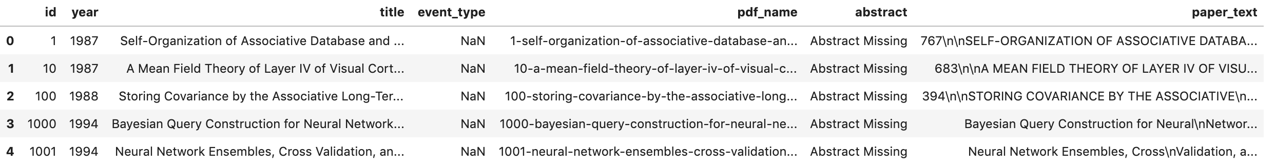
For this tutorial, we’ll use the dataset of papers published in NIPS conference. The NIPS conference (Neural Information Processing Systems) is one of the most prestigious yearly events in the machine learning community. The CSV data file contains information on the different NIPS papers that were published from 1987 until 2016 (29 years!). These papers discuss a wide variety of topics in machine learning, from neural networks to optimization methods, and many more.
Let’s start by looking at the content of the file
# Importing modules
import pandas as pd
import osos.chdir('..')# Read data into papers
papers = pd.read_csv('./data/NIPS Papers/papers.csv')# Print head
papers.head()

Data Cleaning
Since the goal of this analysis is to perform topic modeling, we will solely focus on the text data from each paper, and drop other metadata columns
# Remove the columns
papers = papers.drop(columns=['id', 'title', 'abstract',
                              'event_type', 'pdf_name', 'year'], axis=1)# sample only 10 papers - for demonstration purposes
papers = papers.sample(10)# Print out the first rows of papers
papers.head()
Remove punctuation/lower casing
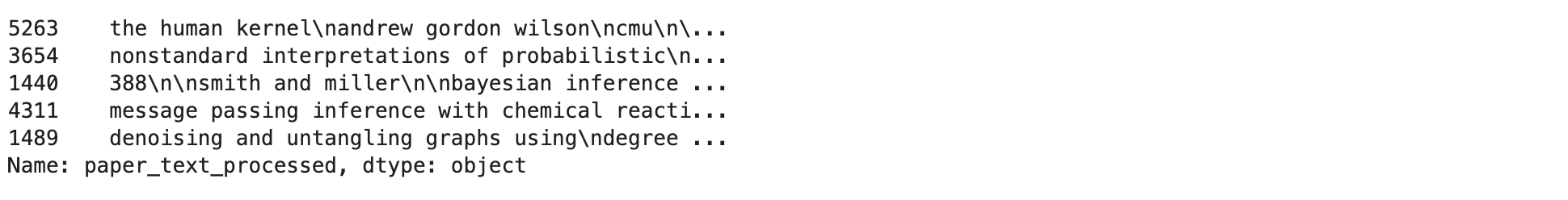
Next, let’s perform a simple preprocessing on the content of paper_text column to make them more amenable for analysis, and reliable results. To do that, we’ll use a regular expression to remove any punctuation, and then lowercase the text
# Load the regular expression library
import re# Remove punctuation
papers['paper_text_processed'] = papers['paper_text'].map(lambda x: re.sub('[,\.!?]', '', x))# Convert the titles to lowercase
papers['paper_text_processed'] = papers['paper_text_processed'].map(lambda x: x.lower())# Print out the first rows of papers
papers['paper_text_processed'].head()

Tokenize words and further clean-up text
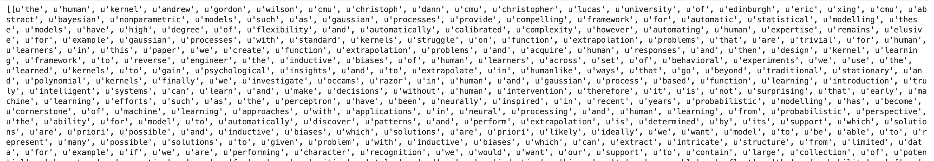
Let’s tokenize each sentence into a list of words, removing punctuations and unnecessary characters altogether.
%%timeimport gensim
from gensim.utils import simple_preprocessdef sent_to_words(sentences):
    for sentence in sentences:
        yield(gensim.utils.simple_preprocess(str(sentence), deacc=True))  # deacc=True removes punctuationsdata = papers.paper_text_processed.values.tolist()
data_words = list(sent_to_words(data))print(data_words[:1])

Phrase Modeling: Bi-grams and Tri-grams
Bigrams are two words frequently occurring together in the document. Trigrams are 3 words frequently occurring. Some examples in our example are: ‘back_bumper’, ‘oil_leakage’, ‘maryland_college_park’ etc.
Gensim’s Phrases model can build and implement the bigrams, trigrams, quadgrams and more. The two important arguments to Phrases are min_count and threshold.
The higher the values of these param, the harder it is for words to be combined.
# Build the bigram and trigram models
bigram = gensim.models.Phrases(data_words, min_count=5, threshold=100) # higher threshold fewer phrases.
trigram = gensim.models.Phrases(bigram[data_words], threshold=100)# Faster way to get a sentence clubbed as a trigram/bigram
bigram_mod = gensim.models.phrases.Phraser(bigram)
trigram_mod = gensim.models.phrases.Phraser(trigram)
Remove Stopwords, Make Bigrams and Lemmatize
The phrase models are ready. Let’s define the functions to remove the stopwords, make trigrams and lemmatization and call them sequentially.
# NLTK Stop words
# import nltk
# nltk.download('stopwords')
from nltk.corpus import stopwordsstop_words = stopwords.words('english')
stop_words.extend(['from', 'subject', 're', 'edu', 'use'])# Define functions for stopwords, bigrams, trigrams and lemmatizationdef remove_stopwords(texts):
    return [[word for word in simple_preprocess(str(doc)) if word not in stop_words] for doc in texts]def make_bigrams(texts):
    return [bigram_mod[doc] for doc in texts]def make_trigrams(texts):
    return [trigram_mod[bigram_mod[doc]] for doc in texts]def lemmatization(texts, allowed_postags=['NOUN', 'ADJ', 'VERB', 'ADV']):
    """https://spacy.io/api/annotation"""
    texts_out = []
    for sent in texts:
        doc = nlp(" ".join(sent))
        texts_out.append([token.lemma_ for token in doc if token.pos_ in allowed_postags])
    return texts_out
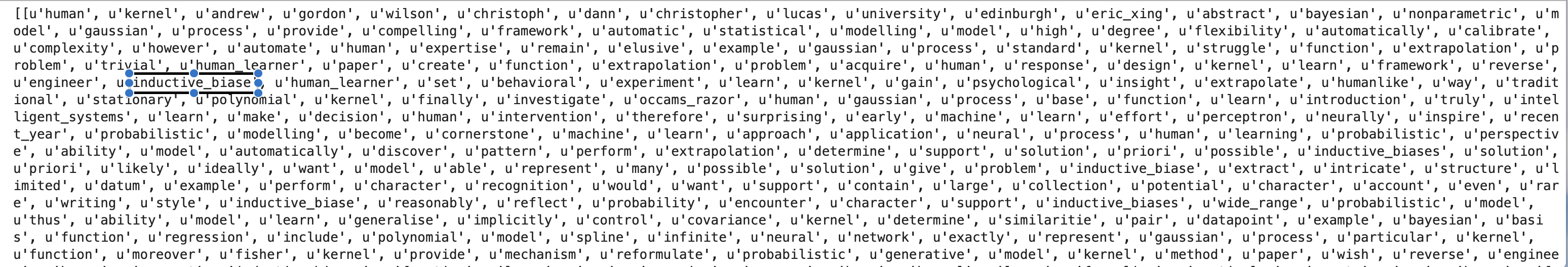
Let’s call the functions in order.
import spacy# Remove Stop Words
data_words_nostops = remove_stopwords(data_words)# Form Bigrams
data_words_bigrams = make_bigrams(data_words_nostops)# Initialize spacy 'en' model, keeping only tagger component (for efficiency)
nlp = spacy.load("en_core_web_sm", disable=['parser', 'ner'])# Do lemmatization keeping only noun, adj, vb, adv
data_lemmatized = lemmatization(data_words_bigrams, allowed_postags=['NOUN', 'ADJ', 'VERB', 'ADV'])print(data_lemmatized[:1])

Data Transformation: Corpus and Dictionary
The two main inputs to the LDA topic model are the dictionary(id2word) and the corpus. Let’s create them.
import gensim.corpora as corpora# Create Dictionary
id2word = corpora.Dictionary(data_lemmatized)# Create Corpus
texts = data_lemmatized# Term Document Frequency
corpus = [id2word.doc2bow(text) for text in texts]# View
print(corpus[:1])

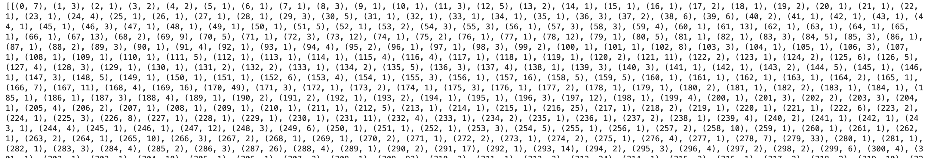
Gensim creates a unique id for each word in the document. The produced corpus shown above is a mapping of (word_id, word_frequency).
For example, (0, 7) above implies, word id 0 occurs seven times in the first document. Likewise, word id 1 occurs thrice and so on
Base Model
We have everything required to train the base LDA model. In addition to the corpus and dictionary, you need to provide the number of topics as well. Apart from that, alpha and eta are hyperparameters that affect sparsity of the topics. According to the Gensim docs, both defaults to 1.0/num_topics prior (we’ll use default for the base model).
chunksize controls how many documents are processed at a time in the training algorithm. Increasing chunksize will speed up training, at least as long as the chunk of documents easily fit into memory.
passes controls how often we train the model on the entire corpus (set to 10). Another word for passes might be “epochs”. iterations is somewhat technical, but essentially it controls how often we repeat a particular loop over each document. It is important to set the number of “passes” and “iterations” high enough.
# Build LDA model
lda_model = gensim.models.LdaMulticore(corpus=corpus,
                                       id2word=id2word,
                                       num_topics=10,
                                       random_state=100,
                                       chunksize=100,
                                       passes=10,
                                       per_word_topics=True)
View the topics in LDA model
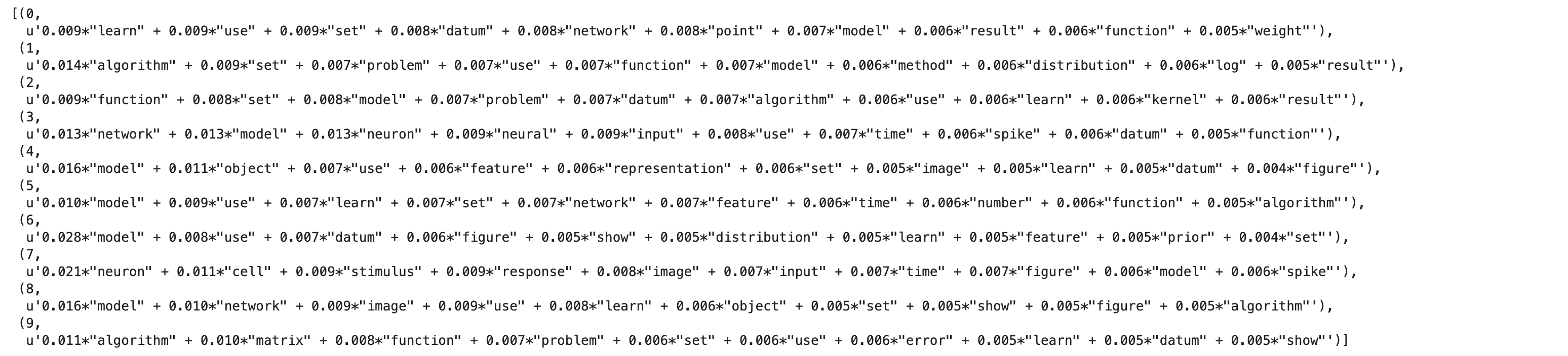
The above LDA model is built with 10 different topics where each topic is a combination of keywords and each keyword contributes a certain weightage to the topic.
You can see the keywords for each topic and the weightage(importance) of each keyword using lda_model.print_topics()
from pprint import pprint# Print the Keyword in the 10 topics
pprint(lda_model.print_topics())
doc_lda = lda_model[corpus]

Compute Model Perplexity and Coherence Score
Let’s calculate the baseline coherence score
from gensim.models import CoherenceModel# Compute Coherence Score
coherence_model_lda = CoherenceModel(model=lda_model, texts=data_lemmatized, dictionary=id2word, coherence='c_v')
coherence_lda = coherence_model_lda.get_coherence()print('\nCoherence Score: ', coherence_lda)
Coherence Score: 0.301
Hyperparameter Tuning
First, let’s differentiate between model hyperparameters and model parameters :
Model hyperparameters can be thought of as settings for a machine learning algorithm that are tuned by the data scientist before training. Examples would be the number of trees in the random forest, or in our case, number of topics K
Model parameters can be thought of as what the model learns during training, such as the weights for each word in a given topic
Now that we have the baseline coherence score for the default LDA model, let’s perform a series of sensitivity tests to help determine the following model hyperparameters:
- Number of Topics (K)
- Dirichlet hyperparameter alpha: Document-Topic Density
- Dirichlet hyperparameter beta: Word-Topic Density
We’ll perform these tests in sequence, one parameter at a time by keeping others constant and run them over the two different validation corpus sets. We’ll use C_v as our choice of metric for performance comparison
# supporting function
def compute_coherence_values(corpus, dictionary, k, a, b):

    lda_model = gensim.models.LdaMulticore(corpus=corpus,
                                           id2word=id2word,
                                           num_topics=10,
                                           random_state=100,
                                           chunksize=100,
                                           passes=10,
                                           alpha=a,
                                           eta=b,
                                           per_word_topics=True)

    coherence_model_lda = CoherenceModel(model=lda_model, texts=data_lemmatized, dictionary=id2word, coherence='c_v')

    return coherence_model_lda.get_coherence()
Let’s call the function, and iterate it over the range of topics, alpha, and beta parameter values
import numpy as np
import tqdmgrid = {}
grid['Validation_Set'] = {}# Topics range
min_topics = 2
max_topics = 11
step_size = 1
topics_range = range(min_topics, max_topics, step_size)# Alpha parameter
alpha = list(np.arange(0.01, 1, 0.3))
alpha.append('symmetric')
alpha.append('asymmetric')# Beta parameter
beta = list(np.arange(0.01, 1, 0.3))
beta.append('symmetric')# Validation sets
num_of_docs = len(corpus)
corpus_sets = [# gensim.utils.ClippedCorpus(corpus, num_of_docs*0.25),
               # gensim.utils.ClippedCorpus(corpus, num_of_docs*0.5),
               gensim.utils.ClippedCorpus(corpus, num_of_docs*0.75),
               corpus]corpus_title = ['75% Corpus', '100% Corpus']model_results = {'Validation_Set': [],
                 'Topics': [],
                 'Alpha': [],
                 'Beta': [],
                 'Coherence': []
                }# Can take a long time to run
if 1 == 1:
    pbar = tqdm.tqdm(total=540)

    # iterate through validation corpuses
    for i in range(len(corpus_sets)):
        # iterate through number of topics
        for k in topics_range:
            # iterate through alpha values
            for a in alpha:
                # iterare through beta values
                for b in beta:
                    # get the coherence score for the given parameters
                    cv = compute_coherence_values(corpus=corpus_sets[i], dictionary=id2word,
                                                  k=k, a=a, b=b)
                    # Save the model results
                    model_results['Validation_Set'].append(corpus_title[i])
                    model_results['Topics'].append(k)
                    model_results['Alpha'].append(a)
                    model_results['Beta'].append(b)
                    model_results['Coherence'].append(cv)

                    pbar.update(1)
    pd.DataFrame(model_results).to_csv('lda_tuning_results.csv', index=False)
    pbar.close()
Investigate Results
Let’s start by determining the optimal number of topics. The chart below outlines the coherence score, C_v, for the number of topics across two validation sets, and a fixed alpha = 0.01 and beta = 0.1

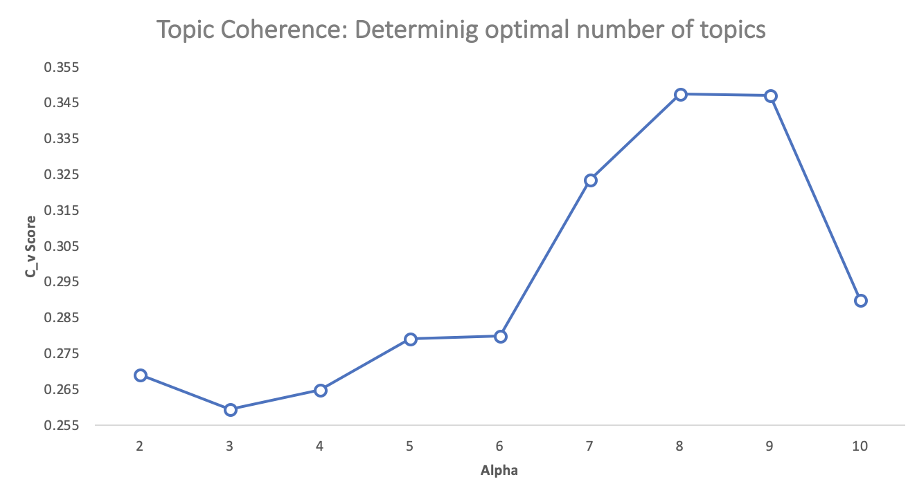
With the coherence score seems to keep increasing with the number of topics, it may make better sense to pick the model that gave the highest CV before flattening out or a major drop. In this case, we picked K=8
Next, we want to select the optimal alpha and beta parameters. While there are other sophisticated approaches to tackle the selection process, for this tutorial, we choose the values that yielded maximum C_v score for K=8

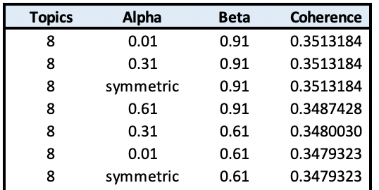
alpha=0.01
beta=0.9
K=8
That yields approx. 17% improvement over the baseline score
Final Model
Let’s train the final model using the above selected parameters
lda_model = gensim.models.LdaMulticore(corpus=corpus,
id2word=id2word,
num_topics=8,
random_state=100,
chunksize=100,
passes=10,
alpha=0.01,
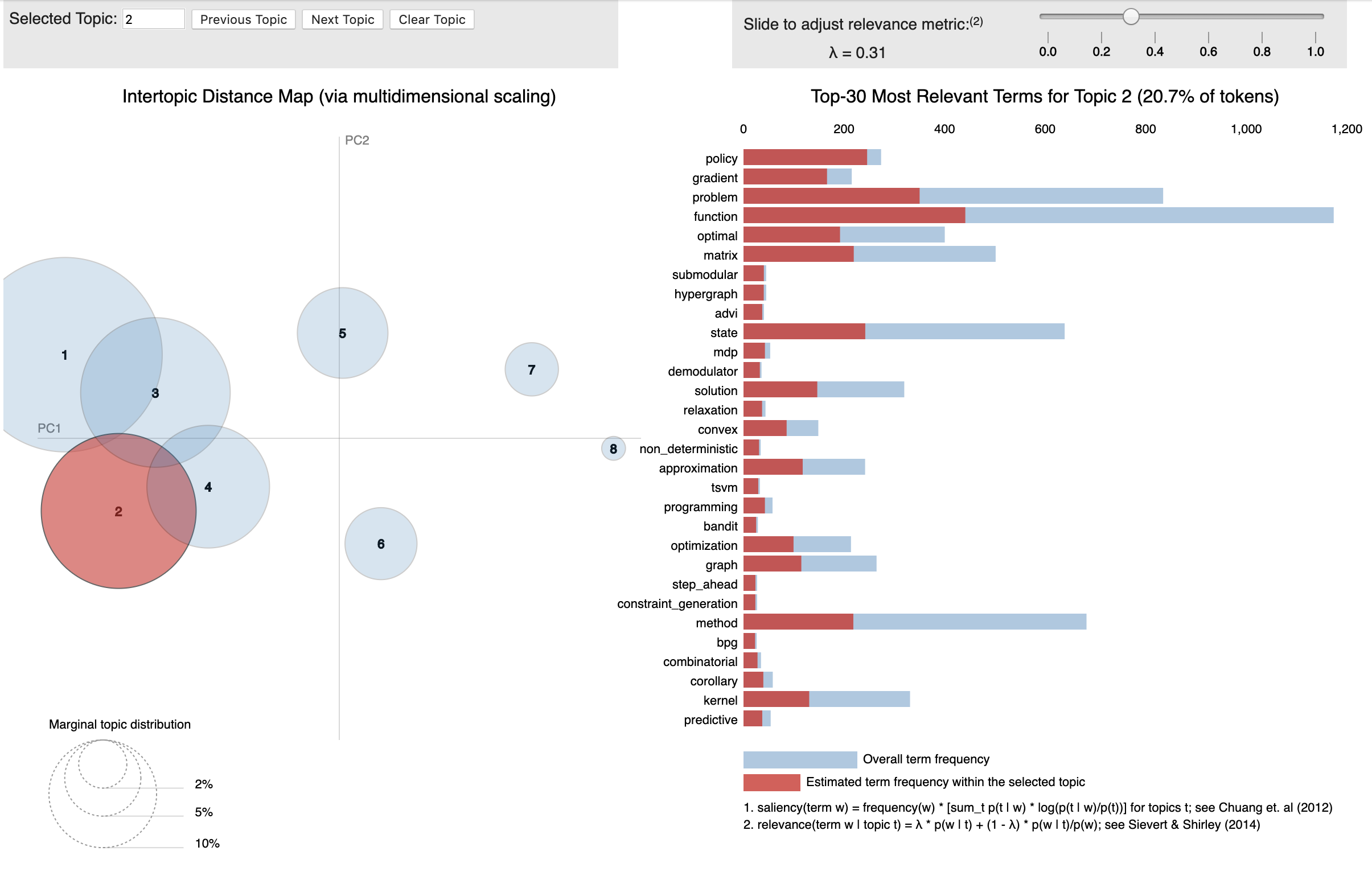
eta=0.9)Visualize Topics
import pyLDAvis.gensim
import pickle
import pyLDAvis# Visualize the topics
pyLDAvis.enable_notebook()LDAvis_prepared = pyLDAvis.gensim.prepare(lda_model, corpus, id2word)LDAvis_prepared

Closing Notes
We started with understanding why evaluating the topic model is essential. Next, we reviewed existing methods and scratched the surface of topic coherence, along with the available coherence measures. Then we built a default LDA model using Gensim implementation to establish the baseline coherence score and reviewed practical ways to optimize the LDA hyperparameters.
Hopefully, this article has managed to shed light on the underlying topic evaluation strategies, and intuitions behind it.
Thanks for reading. If you have any feedback, please feel to reach out by commenting on this post, messaging me on LinkedIn, or shooting me an email (shmkapadia[at]gmail.com)
If you enjoyed this article, visit my other articles
Content from https://towardsdatascience.com/


0 Comments