How, When, and Why Should You Normalize / Standardize / Rescale Your Data?

Before diving into this topic, lets first start with some definitions.

“Rescaling” a vector means to add or subtract a constant and then multiply or divide by a constant, as you would do to change the units of measurement of the data, for example, to convert a temperature from Celsius to Fahrenheit.

“Normalizing” a vector most often means dividing by a norm of the vector. It also often refers to rescaling by the minimum and range of the vector, to make all the elements lie between 0 and 1 thus bringing all the values of numeric columns in the dataset to a common scale.

“Standardizing” a vector most often means subtracting a measure of location and dividing by a measure of scale. For example, if the vector contains random values with a Gaussian distribution, you might subtract the mean and divide by the standard deviation, thereby obtaining a “standard normal” random variable with mean 0 and standard deviation 1.

After reading this post you will know:

• Why should you standardize/normalize/scale your data
• How to standardize your numeric attributes to have a 0 mean and unit variance using standard scalar
• How to normalize your numeric attributes between the range of 0 and 1 using min-max scalar
• How to normalize using robust scalar
• When to choose standardization or normalization

Let’s get started.

Why Should You Standardize / Normalize Variables:

Standardization:

Standardizing the features around the center and 0 with a standard deviation of 1 is important when we compare measurements that have different units. Variables that are measured at different scales do not contribute equally to the analysis and might end up creating a bais.

For example, A variable that ranges between 0 and 1000 will outweigh a variable that ranges between 0 and 1. Using these variables without standardization will give the variable with the larger range weight of 1000 in the analysis. Transforming the data to comparable scales can prevent this problem. Typical data standardization procedures equalize the range and/or data variability.

Normalization:

Similarly, the goal of normalization is to change the values of numeric columns in the dataset to a common scale, without distorting differences in the ranges of values. For machine learning, every dataset does not require normalization. It is required only when features have different ranges.

For example, consider a data set containing two features, age, and income(x2). Where age ranges from 0–100, while income ranges from 0–100,000 and higher. Income is about 1,000 times larger than age. So, these two features are in very different ranges. When we do further analysis, like multivariate linear regression, for example, the attributed income will intrinsically influence the result more due to its larger value. But this doesn’t necessarily mean it is more important as a predictor. So we normalize the data to bring all the variables to the same range.

When Should You Use Normalization And Standardization:

Normalization is a good technique to use when you do not know the distribution of your data or when you know the distribution is not Gaussian (a bell curve). Normalization is useful when your data has varying scales and the algorithm you are using does not make assumptions about the distribution of your data, such as k-nearest neighbors and artificial neural networks.

Standardization assumes that your data has a Gaussian (bell curve) distribution. This does not strictly have to be true, but the technique is more effective if your attribute distribution is Gaussian. Standardization is useful when your data has varying scales and the algorithm you are using does make assumptions about your data having a Gaussian distribution, such as linear regression, logistic regression, and linear discriminant analysis.

Dataset:

I have used the Lending Club Loan Dataset from Kaggle to demonstrate examples in this article.

Importing Libraries:

import pandas as pd
import numpy as np 
import seaborn as sns
import matplotlib.pyplot as plt

Importing dataset:

Let’s import three columns — Loan amount, int_rate and installment and the first 30000 rows in the data set (to reduce the computation time)

cols = ['loan_amnt', 'int_rate', 'installment']
data = pd.read_csv('loan.csv', nrows = 30000, usecols = cols)

If you import the entire data, there will be missing values in some columns. You can simply drop the rows with missing values using the pandas drop na method.

Basic Analysis:

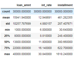
Let’s now analyze the basic statistical values of our dataset.

data.describe()

The different variables present different value ranges, therefore different magnitudes. Not only the minimum and maximum values are different, but they also spread over ranges of different widths.

Standardization (Standard Scalar) :

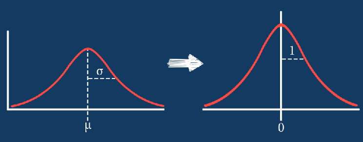
As we discussed earlier, standardization (or Z-score normalization) means centering the variable at zero and standardizing the variance at 1. The procedure involves subtracting the mean of each observation and then dividing by the standard deviation:

The result of standardization is that the features will be rescaled so that they’ll have the properties of a standard normal distribution with

μ=0 and σ=1

where μ is the mean (average) and σ is the standard deviation from the mean.

CODE:

StandardScaler from sci-kit-learn removes the mean and scales the data to unit variance. We can import the StandardScalar method from sci-kit learn and apply it to our dataset.

from sklearn.preprocessing import StandardScaler
scaler = StandardScaler() 
data_scaled = scaler.fit_transform(data)

Now let's check the mean and standard deviation values

print(data_scaled.mean(axis=0))
print(data_scaled.std(axis=0))

As expected, the mean of each variable is now around zero and the standard deviation is set to 1. Thus, all the variable values lie within the same range.

print('Min values (Loan Amount, Int rate and Installment): ', data_scaled.min(axis=0))
print('Max values (Loan Amount, Int rate and Installment): ', data_scaled.max(axis=0))

However, the minimum and maximum values vary according to how spread out the variable was, to begin with, and is highly influenced by the presence of outliers.

Normalization (Min-Max Scalar) :

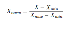
In this approach, the data is scaled to a fixed range — usually 0 to 1.
In contrast to standardization, the cost of having this bounded range is that we will end up with smaller standard deviations, which can suppress the effect of outliers. Thus MinMax Scalar is sensitive to outliers.

A Min-Max scaling is typically done via the following equation:

CODE:

Let’s import MinMaxScalar from Scikit-learn and apply it to our dataset.

from sklearn.preprocessing import MinMaxScaler
scaler = MinMaxScaler() 
data_scaled = scaler.fit_transform(data)

Now let’s check the mean and standard deviation values.

print('means (Loan Amount, Int rate and Installment): ', data_scaled.mean(axis=0))
print('std (Loan Amount, Int rate and Installment): ', data_scaled.std(axis=0))

After MinMaxScaling, the distributions are not centered at zero and the standard deviation is not 1.

print('Min (Loan Amount, Int rate and Installment): ', data_scaled.min(axis=0))
print('Max (Loan Amount, Int rate and Installment): ', data_scaled.max(axis=0))

But the minimum and maximum values are standardized across variables, different from what occurs with standardization.

Robust Scalar (Scaling to median and quantiles) :

Scaling using median and quantiles consists of subtracting the median to all the observations and then dividing by the interquartile difference. It Scales features using statistics that are robust to outliers.

The interquartile difference is the difference between the 75th and 25th quantile:

IQR = 75th quantile — 25th quantile

The equation to calculate scaled values:

X_scaled = (X — X.median) / IQR

CODE:

First, Import RobustScalar from Scikit learn.

from sklearn.preprocessing import RobustScaler
scaler = RobustScaler() 
data_scaled = scaler.fit_transform(data)

Now check the mean and standard deviation values.

print('means (Loan Amount, Int rate and Installment): ', data_scaled.mean(axis=0))
print('std (Loan Amount, Int rate and Installment): ', data_scaled.std(axis=0))

As you can see, the distributions are not centered in zero and the standard deviation is not 1.

print('Min (Loan Amount, Int rate and Installment): ', data_scaled.min(axis=0))
print('Max (Loan Amount, Int rate and Installment): ', data_scaled.max(axis=0))

Neither are the minimum and maximum values set to a certain upper and lower boundaries like in the MinMaxScaler.

I hope you found this article useful. Happy learning!

References

1. https://www.udemy.com/feature-engineering-for-machine-learning/
2. https://www.geeksforgeeks.org/python-how-and-where-to-apply-feature-scaling/